Five Excel Table Shortcuts worth Knowing

 

          Five Excel Table Shortcuts worth Knowing

 

1.    CTRL+T (or: CTRL+L a lesser-known shortcut):
Creates a table

2.    CTRL+SHIFT+8 (CTRL+*):
Selects the entire table,
including the header row and the total row (if present)

3.    CTRL+SHIFT+T (a toggle shortcut):
Adds/removes the total row

4.    CTRL+A:
Selects the entire table, without the total row (if present)

5.    CTRL+SHIFT+drag mouse:
Duplicates the entire table

 

 

 

 

 

 

Excel - 4 methods to copy a cell N times (according to parameter)

 

Excel - 4 methods to copy a cell N times (according to parameter)

 

In this post I'm going to show you 4 different methods to copy a cell's value

And duplicate it N times (N is a parameter)

 

                                                                          Method 1

 

                                                                          Method 2

                                                                         Method 3

 

                                                                          Method 4

 

Excel - Find the most recent visit date of your patients

 

Excel - Find the most recent visit date of your patients

A friend of mine, who is a doctor, came to me seeking help with a problem in Excel.
He said: "I have this list of patients and their visit dates, all mixed up in an unsorted list.

I want to know, for each patient, which is his/her most recent visit date.
And I'd prefer the simplest method in Excel since I don't want to use complicated formulae.

Can you please help me?"

So here is the data:

Pic No.1: Original List

And here a simple solution using a Pivot Table:

 

Pic No.2: Pivot Table Solution

Excel – Intersection: Part II

 

 

Excel – Intersection: Part II

 

In the previous installment I introduced the INTERSECTION feature in Excel. We saw some neat, simple solutions to analysing data gathered from 4 US states over a period of 12 months.         

In this installment, I'm going to show the combination of the Intersection operation with other Excel functions.

Again, these examples will demonstrate the ease of use and the advantage over more "traditional" methods.

 

Example 1: Second smallest number (State and value)

Pic 1: second smallest number of cases in August

Example 2: Intersection & OFFSET

 

          Pic 2: Intersection & OFFSET (NY without the first 2 months)

 

 

Example 3: Intersection & FILTER

         Pic 3: Intersection & FILTER (CA, only cases > 5000)

  

Example 4: Intersection & SORT

 

   Pic 4: Intersection & SORT (Asc. order, TX) with matching months

 

Example 5: 5 last months of FL

                    Pic 5: Last 5 months in FL

 

Excel - What is Intersection? Why is it useful? - Part I

 

 

Excel – Intersection: What is it? Why is it useful?

 

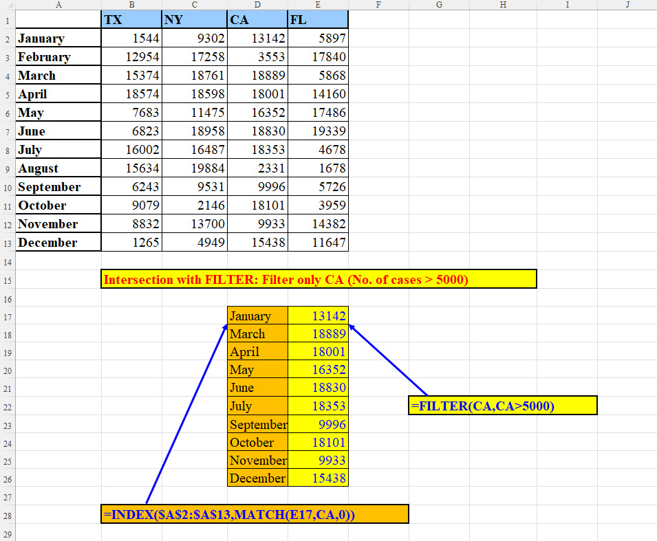
The following dataset displays the number of juvenile delinquency cases opened in four US states during the year 2020. (not really, the data are fabricated 😊 )

Pic 1: the dataset

 

Now, suppose you want to analyse the dataset. For example:
How many cases were opened in Californian in May?

This can easily be solved in various methods,
for example, with the following formula:

                                      Pic 2: A "traditional" solution

Or with this one:

                             Pic 3: Another "traditional" solution

 

 

 

However, there's a far better, much simpler method in Excel for cross tab data.

Unfortunately, it is lesser known. It is called Intersection.
The intersection Operation is ideal when dealing with cross tab data: a column data intersecting a row data.

The intersection operation does not refer to cells or ranges, but to names.

So, how do we use this feature?

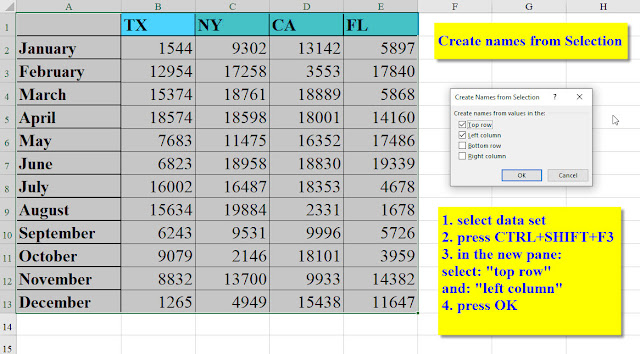
First of all, we need to define the names (taken from cells B1:E1, the column   headers and from cells A2:A13, the row headers)

 

So, we Create names from selection as explained in the picture:      

                                Pic 4: Create Names from Selection    

 

If we take a close look at the definitions created in the Name Manager, we can clearly see that each State has 12 values (the values of the 12 months) and that each month has four values (one for every state).

                            Pic 5: Name Manager's definitions

 

And now let's turn to some cool applications of Intersection.

Example No.1:
Remember the question we asked ourselves at the beginning?
How many cases were opened in Californian in May?

So, instead of a lengthy formula, we can have the solution in a very short formula:
=CA May

          Pic 6: How many cases were opened in California in May

The formula consists of two elements: the column (CA) and the row (May), separated by the intersection operator " ".

So simple, so easy, so obvious….

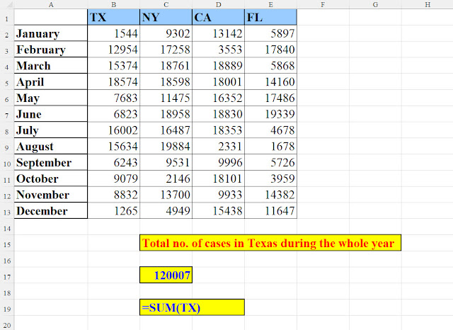
Example No.2:

 

How many cases were opened in Texas alone during the entire year?

Pic 7: How many cases were opened in Texas during the entire year?

 

 

Example No.3:

How many cases were opened in Texas in the first 4 months?

      Pic 8: How many cases were opened in Texas during Jan.-Apr.?

 

Example No.4:

How many cases were opened in Texas and California in the first 4 months?

         Pic 9: No. of cases opened in Texas & California in Jan-Apr

 

Example No.5:

How many cases were opened in January (excluding Texas)?

   Pic 10: How many cases were opened in January (excluding Texas)

 

Example No.6:

Total cases in Texas, California and Florida (altogether)

      Pic 11: Total cases in Texas, California and Florida (altogether)

 

 

 

How to remove empty rows in a range (without VBA, without PQ, without formulae, even without the mouse)

 

Excel – How to remove empty rows in a range

 

The following technique explains, step by step, how to get rid of empty rows within a range.

Please note that this technique does not use either VBA, PQ or formulae.

It doesn't even use the mouse 😊

How to get rid of unwanted names in a list

 

How to get rid of unwanted names in a list

(no formulae, no PQ)

Suppose you have a list of names (in col. A) from which you need to exclude names that appear in a different list (col. C)

 

This can be easily done in a few simple steps without formulae or Power Query:

 

A .  we prepare two lists

In col. A – the original list

In col. C – the list of names to exclude from the original list.

                                                    Pic No.1

 

B .  we "color" in yellow all the names in col. A

                                                            Pic No.2

 

 

C.  Find duplicates using Conditional Formatting
select both columns-> Conditional Formatting-> Highlight Cells Rules->Duplicate Values

 

 

                                                Pic No.3

 

D. Filter the list in col. A and select: Filter by cell color.

You should, of course, select the yellow color

                                                     Pic No.4

E. Final Result: now the list in col. A contains only names that do not appear in the list of col. C

 

                                                                Pic No.5