Extracting Country Name from End of String

Extracting Country Name from End of String

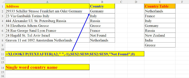
Suppose you have a list of addresses, where the country name appears at the end and you need to check whether the name appears in a country table.

This can easily be done, for example, by extracting the last word of the string and using XLOOKUP to verify that this is indeed a valid country name.

 

                   Pic 1: Extract Country Name from End of String

 

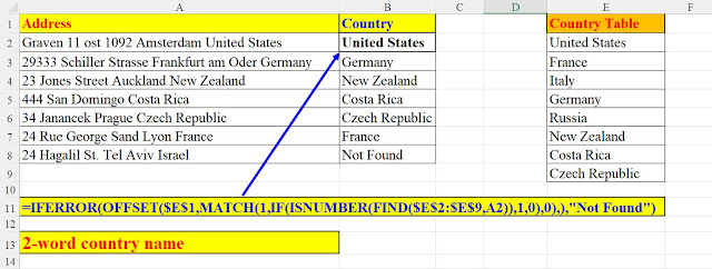
But what if the country name consists of two words and not just one?
For example: United States, United Arab Emirates, Ivory Coast, Czech Republic, New Zealand…..?

Then, the previous solution won’t always work.

So, we found a better solution for countries with more than one word in their names.

Pic 2: Country Name consists of one or more words

 

This solution has (at least) three advantages:

1.      It can be applied in any Excel version, not only in Excel 365

2.     As stated above, it can handle countries whose names consist of more than one word

3.    Unlike the first solution, where the country name must be at the end of the string, the second solution allows us to find countries in the middle of the string.

 

 

  

 

A new Method to analyze financial data

What I’m going to share with you today is a trick I invented when analyzing financial data: general ledger, balance sheet... The exact term isn’t important as long as you analyze….money.

So, here’s the trick:

Suppose you want to find out the sum of several months: could be a full year, could be 6 months, could be a quarter… you name it.

So, the idea is to have 3 parameters that control the process:

1.       The column to start with

2.       How many consecutive columns do I want to sum up

3.        What line do I want to analyze

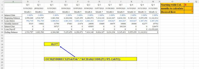
                    Example No.1: Summing Cells B7:C7

 In this example, we want to sum up the monthly interest of the first two months of the year: columns B and column C.

 So, the result appears in cell D14 and the formula – in D19.

And the formula is:
=SUM(INDIRECT(P1&P3&":"&CHAR(CODE(P1)+P2-1)&P3))

The INDIRECT Function constitutes the range B7:C7 in a clever way. How?
The first part of the range(“B7”) is created by concatenating the starting column (“B”) [first parameter - P1] with the desired row (“7”) [third parameter - P3].

The second part of the INDIRECT is the more interesting one: we convert the letter “B” (of the first parameter) into its ASCII code: 66, and add the numbers of months to calculate (2) [second parameter - P2], then we subtract one: we need to add only 1 in order to calculate two months.

The number created in this summing process is 67.
Now we convert this number back into an ASCII letter (“C”) and we concatenate it with the row number (“7”) exactly as we did in the first part.

The string created (“B7:C7”) is then summed up, and the result: 18977 is the sum of B7 (8315) and of C7 (10662).

 

Let’s take another example:

                        Example No.2: Summing Cells E5:C5

 

Here we want to sum the second quarter of the year (months: 4,5,6 in columns F,G,H) for row no.5

So, the INDIRECT’s string in this case would be: “E5:G5”, and the sum of these cells amounts to the sum in cell D14: 4164046+5225459+6286873=15676377

 

 

 

Excel 365 - Four Methods to extract only Digits from a String

 Excel 365 - Four Methods to extract only Digits from a String

 

There are, of course, numerous ways to extract only digits from a string of characters.
Today I’m going to show only four and only in Excel 365.

All methods use the SEQUENCE function, an indispensable function when “breaking” a string into its “atoms”.

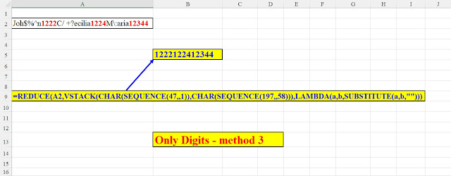
The third one is using LAMBDA with the brand new REDUCE function.

 

Method 1 – using CONCAT

Method 2 – using TEXTJOIN

Method 3 – REDUCE with a LAMBDA

Method 4 – CONCAT with ISNUMBER