A new Method to analyze financial data
What I’m going to share with you today is a trick I invented
when analyzing financial data: general ledger, balance sheet... The exact term
isn’t important as long as you analyze….money.
So, here’s the trick:
Suppose you want to find out the sum of several months: could
be a full year, could be 6 months, could be a quarter… you name it.
So, the idea is to have 3 parameters that control the
process:
1.
The column to start with
2.
How many consecutive columns do I want
to sum up
3.
What line do I want to analyze
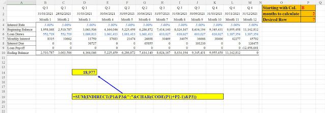
Example No.1: Summing Cells B7:C7
And the formula is:
=SUM(INDIRECT(P1&P3&":"&CHAR(CODE(P1)+P2-1)&P3))
The INDIRECT Function constitutes the range B7:C7 in a clever
way. How?
The first part of the range(“B7”) is created by concatenating the starting column
(“B”) [first parameter - P1] with the desired row (“7”) [third parameter - P3].
The second part of the INDIRECT is the more interesting one: we convert the letter
“B” (of the first parameter) into its ASCII code: 66, and add the numbers of
months to calculate (2) [second parameter - P2], then we subtract one: we need to add only 1 in order
to calculate two months.
The number created in this summing process is 67.
Now we
convert this number back into an ASCII letter (“C”) and we concatenate it with
the row number (“7”) exactly as we did in the first part.
The string created (“B7:C7”) is then summed up, and the result:
18977 is the sum of B7 (8315) and of C7 (10662).
Let’s take another example:
Example No.2: Summing Cells E5:C5
Here we want to sum the second quarter of the year (months:
4,5,6 in columns F,G,H) for row no.5
So, the INDIRECT’s string in this case would be: “E5:G5”, and the sum of these cells amounts to the sum in cell D14: 4164046+5225459+6286873=15676377


אין תגובות:
הוסף רשומת תגובה