10+ methods to zoom in or out in Excel

10+ methods to zoom in or out  in Excel

Excel has a great visibility enhancement tool: the zoom-in/zoom-out feature.
Zooming (in or out) in an Excel sheet is very useful.
You can zoom out (minimize the sheet size) down to 10% and zoom in (maximize the sheet size) up to 400%.

 

Pic 1: default zoom: 100%

 

Pic 2: maximum zoom-out: 10%

 

Pic 3: maximum zoom-in: 400%

This post will demonstrate ten(!) methods of zooming (in or out)

1)           CTRL+Mouse wheel – Press CTRL & scroll the mouse wheel. If you scroll the wheel upwards, it zooms in. if you push it downwards, it zooms out. The main problem with this method is that you cannot stop at an exact desired size.

 

2)           By customizing the status bar you'll be able both to control the sheet's zoom and to display the zoom percentage

Pic 4: Customizing the Status Bar

 

 

 

Dragging the zoom slider on the rightmost corner of the screen. Sliding to the right – increases the sheet’s size, whereas sliding to the left - decreases the sheet's size.
Same problem as in the previous method: it is difficult to stop at an exact desired value.

Pic 5: Using the slider on the Status Bar

 

 

3)           Activating the Zoom pane with the keyboard shortcut: ALT, W, Q

Here, you can either choose a predefined value corresponding to the radio button. Or you can fit the selection by typing your desired size ( a number between 10 and 400).
Choosing (or Typing) a number smaller than the actual sheet size will decrease the sheet’s size, however a number greater than the actual sheet size will increase the sheet's size.

Pic 6: ALT+W+Q and Choose the desired value

 

4)           Activating the Zoom pane with the keyboard shortcut: ALT, V, Z

Same as the previous method.

Pic 7: ALT+V+Z and Choose the desired value

 

5)           Instead of the above-mentioned two shortcut key methods, you can simply click the View tab, then click the ZOOM icon within the zoom group (the leftmost icon) . This will open the same pane as with shortcuts: ALT, W, Q (method 3) or ALT, V, Z (method 4)

 

 

Pic 8: accessing the zoom icon from the View tab      

                

6)           Clicking the View tab and then the 100% icon within the zoom group (second in this group). This will reset the sheet’s size to the default 100%.

Pic 9: View tab - setting the default zoom

 

7)           If you prefer to use the keyboard instead of the mouse, the same effect (resetting the sheet’s size to the default 100%.) can be achieved with this keyboard shortcut: ALT, W, J

 

8)           Zoom to selection: If you want to have maximum zoom on a certain range (400%), select the range and then press:
ALT, W, G.

Or: Click the View Tab and then the Zoom to Selection icon on the Zoom group (rightmost icon)

 

Pic 10: View – Zoom to Selection

The same result will be achieved if you add the “Zoom to Selection” icon to your QAT.    

 

9)           the keyboard combination of ALT+CTRL++  zooms the screen in, and: ATL+CTRL+-  zooms out

10)      Add the Zoom in and Zoom out commands to QAT

The Zoom In can increase the size up to 200%.

The Zoom out can decrease the size down to 25%.

 

11)      Add 2 icons/shapes and assign a macro.

in order to increase the screen by 10% each time you click the icon, add this macro:
Sub Zoom_IN()
    ActiveWindow.Zoom = ActiveWindow.Zoom + 10
End Sub

in order to decrease the screen by 10% each time you click the icon, add this macro:
Sub Zoom_OUT()
    ActiveWindow.Zoom = ActiveWindow.Zoom – 10
End Sub

          

Pic 11: Shapes & Macros to Zoom in/Zoom out

 

I have added 6 icons to my QAT.

From left to right:
* Zoom in – as explained in method 9

* zoom out – as explained in method 9

* “classic” zoom – this icon has 6 predefined options:

200%, 100%, 75%, 50%, 25% and Selection. Choosing “Selection” will increase the sheet’s size to its maximum = 400%

*  zoom to selection - will increase the sheet’s size to its maximum = 400%

* zoom “dialog” – clicking this icon will display the same pane as in methods 3 & 4 (the keyboard shortcut keys: ALT, W, Q or ALT, V, Z)

* “group” zoom – clicking this icon will display the same three icons of the View->Zoom group:
Zoom, 100% and Zoom to Selection.

Pic 12: Zoom icons on my QAT

Please note that the third, fifth and sixth icons are identical. Only by hovering the mouse over the icon, will you be able to notice the different functionality. This is, undoubtedly, quite confusing.

To sum up: There are many ways to zoom in or out the sheet’s size. As always, in Excel you can achieve the same goal via more than one way:
-   Clicking the icon on the ribbon
-   Clicking the icons that were added to QAT
-   Using keyboard shortcuts
-   Using the mouse
-   Dragging the zoom slider
-   VBA

 

 

         

Don’t use FIND/SEARCH, use this approach instead

 

Don’t use FIND/SEARCH, use this approach instead

Surprised by the article’s title?

Here’s the scenario:

You own a restaurant and you have some waiters working on 3 different shifts: morning, noon, evening.
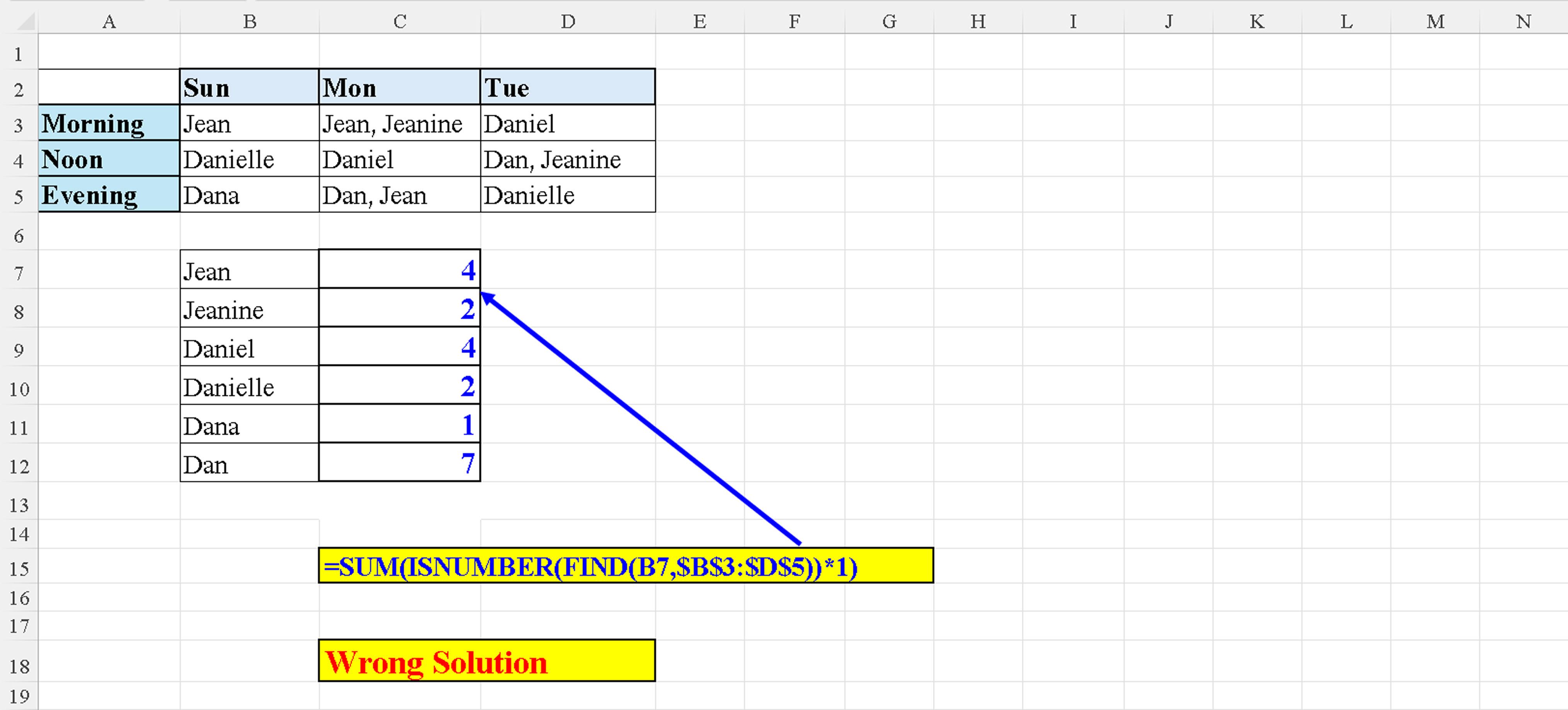
You want to know, for a certain period of time (say: Sunday, Monday and Tuesday), how many assigned shifts did each waiter have during that period.

You might be tempted to do this:

                   Pic 1: Wrong Solution

As can be seen clearly, this is a wrong solution:
Jean does not appear 4 times in the list, but only 3.
Dan does not appear 7 times in the list, but only twice.
So, what is the root of the problem?
The name “Jean”, for example, is contained within “Jeanine”. So the FIND function finds the substring “Jean” 4 times in the list.

The name “Dan” is contained in “Dana”, “Daniel” and “Danielle”, so the FIND function fetches all the instances of the substring “Dan” within the list.

Here we can see another shortcoming of the FIND function.
If, for example, we have “Jean” twice in cell C3, the formula:

=SUM(ISNUMBER(FIND(B7,C3)*1)

Will return a wrong result: 1 instead of 2.

FIND stops short of finding all the instances of the searched string within the cell.

                   Pic 2: Wrong Solution (a single cell)

 

So, you’d  probably ask, what is the solution to this problem?
The answer is: use EXACT instead of FIND.

The formula is a bit longer but by using the EXACT function we get the exact solution.

                   Pic 3: Correct Solution

 

 

And as a “bonus”, if the name “Jean” appears twice in cell C3, the EXACT function returns the correct result, unlike the FIND function (as demonstrated above):

                   Pic 4: Correct Solution (a single cell)

 

 

 

 

Combine data from multiple sheets without PQ

 

Combine data from multiple sheets without PQ

We all know that Power Query is the ideal tool to combine data from multiple tables/sheets/files etc.
But sometimes one can use a simpler, faster solution. This solution will still work even if the data changes.

Consider the following scenario:
I and some friends are planning on a four-day camp in the desert. We have prepared the list of products and quantities per product for each day. In order to buy these products, we need to find out the total quantity for each product that we are going to consume in our trip. Of course, some items might repeat themselves in several days. And of course, as stated above, we want the solution to be dynamic: if you add/delete a product, or if you modify a product’s quantity, we want this to be reflected in the purchase list.

So here’s the data, in 4 sheets: Day1 to Day4

                        Day 1: Products and Quantity

                        Day 2: Products and Quantity

 

 

                        Day 3: Products and Quantity

 

                        Day 4: Products and Quantity

 

We have two solutions, using VSTACK

Solution 1:
1) Create a dynamic array of all the data in all four sheets.
2) Use this array in a pivot table. All the “empty” rows of array are grouped into one row in the pivot table.

    The Pivot Table uses the array created by VSTACK

 

3) This “0” row of the Pivot Table can easily be eliminated by filtering it out.

        The Pivot Table after filtering out the “0” row

 

 

Solution 2:

Using both VSTACK and the new GROUPBY functions, we can achieve the same in one formula.
The same method may be employed to get rid of the “0” row (or even the “total” row if you omitted the 4^th argument to the GROUPBY function).

        VSTACK & GROUPBY instead of Power Query

 

 

 

Twenty KB shortcuts In Excel 365 using the SHIFT key

Excel 365 - 20 KB shortcuts using the SHIFT key

1.  SHIFT+PAGE UP

Extends selection one screen upwards. For example, if your active cell is N31, this action selects cells N1:N31.

 

2. SHIFT+PAGE DOWN

Extends selection one screen downwards. For example, if your active cell is C1, this action selects cells C1:C31.

 

3. SHIFT+HOME

Selects from active cell to first column on the same row. For example, if your active cell is G4, this action selects cells A4:G4.

 

4. SHIFT+SPACEBAR/CTRL+SPACEBAR

In a table:

a. Pressing SHIFT+SPACEBAR when the active cell is in a table – selects the entire record.

b. If you now press CTRL+SPACEBAR - selects the entire table

c. you can select the whole table by pressing: CTRL+SHIFT+SPACEBAR in any cell within the table

 

Outside a table:

a. Pressing SHIFT+SPACEBAR when the active cell is not in a table - selects the entire row.

b. Pressing CTRL+SPACEBAR when the active cell is not in a table - selects the entire column.

c. you can select the whole sheet by pressing: CTRL+SHIFT+SPACEBAR in any cell in the sheet.

 

5. SHIFT+F11

Inserts a new worksheet

6. ALT+SHIFT+F1

Inserts a new worksheet (same as 5.)

7. CTRL+SHIFT+9
Unhides hidden rows within selection

 

8. SHIFT+F7
Opens the Thesaurus pane

  

9. CTRL+SHIFT+F1 (toggle)
Hides/unhides the Title bar, QAT (Quick Access Toolbar), Menu bar and Ribbon

 

10. SHIFT+F6 (or: F6)
Toggles between: Menu bar, Active sheet and Name box

  

11. CTRL+SHIFT+F6
Toggles between open workbooks (when two or more workbooks are open).

 

12. CTRL+SHIFT+O
Select all cells with comments 

 

13. CTRL+SHIFT+Home
Extends selection from the active cell to A1. For example, if the active cell is G17,the range: A1:G17 is selected.

 

14. END->SHIFT->Home
Selects the last non-empty cell in the sheet

15. END->SHIFT->Enter
Selects the intersection of the last non-empty column in the sheet
with the active cell’s row.

For example, if the active cell is A19 and the last non-empty cell is S26, then this keyboard combination will select cell: S19.

16. SHIFT+BACKSPACE
Selects the first cell In a selected range

17. CTRL+SHIFT+[
Selects all Precedents (Direct & Indirect)
(same as: Formulas->Formula Auditing-> Trace Precedents, but without the arrows)

18. CTRL+SHIFT+]
Selects all Dependents (Direct & Indirect)
(same as: Formulas->Formula Auditing-> Trace Dependents, but without the arrows)

19. SHIFT+Enter
After entering a cell address in the Name Box, selects the entire range: from the active cell to the cell whose address was entered in the Name Box.(for example, if your active cell is A2 and you key: A20 in the Name Box and then press SHIFT+Enter – Excel selects the range A2:A20)

20. SHIFT+F2
Adds a new comment/edits an existing comment in the active cell (bear in mind: this refers to “comments”, not to “notes” which are new to Excel 365).

 

Excel - How to create an Index Worksheet

 

How to Create an Index Worksheet
(Easy access to any worksheet in your workbook)

Sometimes your workbook has dozens of sheets and you want to easily navigate to a certain sheet without scanning through the entire list.

In that case, you need to build an INDEX sheet that will facilitate this process and save you a great amount of time.

1)    Create a new worksheet whose name is INDEX and make it the first worksheet of the workbook.

2)    Define a named range in the Name Manager. I called mine “TabNames” but you can choose any valid name.

In the “Refers to” text box, add this formula:

=LET(a, GET.WORKBOOK(1),MID(a, FIND("]",a)+1,255))  

         Pic 1: defining the TabNames formula in the Name Manager

 

          Pic 2: the TabNames formula in the Name Manager

3)    In cell A1 type:

=TRANSPOSE(TabNames)

This will create the list of the file’s sheets in column A, starting from cell A2

   Pic 3: creating the list of sheets in column A

 4)    Type the following formula in cell B2: =HYPERLINK("#"&A2&"!A1")

This formula adds the hyperlink to the worksheet whose name appears in the adjacent cell (A2).

 

          Pic 4: Adding the hyperlink for the first sheet

 5)    Double-click the lower right corner of cell B2 to propagate the formula to the rest of the list

                   Pic 5: Adding the hyperlinks to all the file’s worksheets

Now you’re good to go. Whenever you want to “jump” to a specific worksheet, click the cell in column B in order to go directly to that worksheet.

6)    Don’t forget to update the list whenever you add/modify/delete a worksheet. After each modification you need to refresh the list (select cell A1, press F2 and then: Enter)

And one more trick:

In order to return quickly to the INDEX sheet, define a shortcut name in the Name Manager’s Defined Names, for example: O, which refers to  Cell A1 in your INDEX sheet, as can be seen in this screenshot:

Pic 6: Adding the shortcut key to return to the INDEX sheet

 Now, whenever you want to go back to the INDEX sheet, Press F5 (or: CTRL+G) to display the GO TO pane, type: O In the Reference Text Box and press: OK

Pic 7: going back to the INDEX sheet

This will take you immediately back to the INDEX worksheet.

***

BTW, since the file contains a Macro 4.0 command, you’ll have to save it as a macro-enabled workbook (.xlsm) instead of a regular workbook (.xlsx)