Three methods to display a workbook's named ranges

Sometimes, when your workbook has many named ranges, you'd like to have them as a list, in a separate worksheet.

There are at least three methods to accomplish this task:

1.   The shortest method

1)    Press: the F3 key.
the following pane appears:

Pic 1: Press F3

 

2)    Now, press: ALT+L (or just click the Paste List button)
All the named ranges will be pasted into the worksheet.

 

2.   Using a defined name in the Name Manager

 

1)      Press: CTRL+F3 to get to the Name Manager

2)    Click: New (or press: ALT+n) to define a new name

3)    In the Name textbox enter: List (or any name you like)

4)    In the Refers to textbox enter: =NAMES()

Pic 2: define a named range that refers to the NAMES() command

 

5)    In an empty cell of the worksheet, type:
=TRANSPOSE(List) 

All the workbook names will be pasted into the worksheet.

 

3.   VBA

Add the following code to the VBA editor and run it:

Pic 3: Add this code to the VBA editor and run it

 

After running the code you'll see the list of all the workbook's names in a new worksheet.

 

How many active months

 

How many active months

A client of mine came to me with this problem:

Once a year he gets a yearly activity of items. Since the data is sent from a legacy system, Each item's activity is represented by a 24-character string which contains only digits. Each two digits represent a month, so we have 12 consecutive months in each data item,
as can be seen in the picture (the data are painted for better visibility) 

Pic1: the raw data – each 2 digits represent a month

The problem:
We want to know, from the year, how many months yielded an activity.
If the 2-digits are "00", then there was no activity in that month.
Otherwise, that month had an activity and should be counted.

The solution can be achieved with one formula:

Pic 2: Solution in one formula

 

The formula can be better understood by splitting it into two parts:

Part 1:
create an array of 12 horizontal cells, each cell for a month.

This can easily be accomplished with my favourite function: SEQUENCE.

The multiplication by 1 converts the text digits into "real" numbers.

Pic 3: Part 1 of the solution – creating a numeric array of 12 months

Part 2:

Using any method of conditional counting, to count only non-zero numbers in the array. This can be done in several ways.

For example:

1)   Using the same formula of Part 1 and wrapping it with: SUM(IF(…..),1,0)

 

Pic 4: Part 2 of the solution – the same formula

 

2)   COUNTIF with the spilled array

 

Pic 5: Part 2 of the solution – two formulae

 

 

 

 

Add any number of empty rows to a range

Add any number of empty rows to a range

 

This is a sequel to my original post:
Add alternate empty rows to a range – the coolest method

https://meniporat.blogspot.com/2022/08/add-alternate-empty-rows-to-range.html

 

After publishing it, I thought:

Why not create a generic solution?
Why add only 1 row? Why not 2 or 3 or more?
So I came up with a Parameterized solution:

Put the desired number of empty rows in one formula.

And lo and behold, you have it, like magic.

Attached are three pictures, demonstrating my generic solution:
The first, only one empty row  

The second, two empty rows

The third, three empty rows.

Enjoy 😊

Pic 1 - Add one empty row

 

 

Pic 2 - Add two empty rows

 

 

Pic 3 - Add three empty rows

Add alternate empty rows to a range – the coolest method

Add alternate empty rows to a range – the coolest method

 

Suppose you have a range of consecutive data in column A and you want to add alternate empty rows between the range's cells.

How can this be done in the shortest, most elegant way?

Well, there are several methods to accomplish this task.

For example, here:
https://www.myofficetricks.com/how-to-insert-alternate-blank-rows-in-excel-spreadsheet/

Or here:
https://www.extendoffice.com/documents/excel/3727-excel-paste-in-alternate-rows.html

 

But they are all time-consuming because they demand several steps.

Here's the coolest method, that uses only one formula:

 

 

 

  

Shortest method to navigate to a worksheet

 

Shortest method to navigate to a worksheet

 

Your workbook is huge. It has dozens of sheets. After working in a certain sheet you need to return to the Master sheet/Index sheet or whatever name you call it.

You could, of course, add a hyperlink to the master sheet from each and every sheet but that, of course, isn't practical.

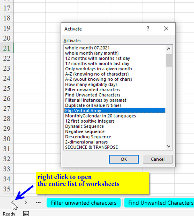
On the other hand, the "classical" method (as shown in the next two pictures) is also a cumbersome and time-consuming two-phase process.

    

            Old method 1: right-click the navigation icon < to display the worksheets' list

 

                    Old method 2: scroll through the list. When you reach the sheet press OK

 

So what's the best solution?

Creating a named range and using it with one click 😊

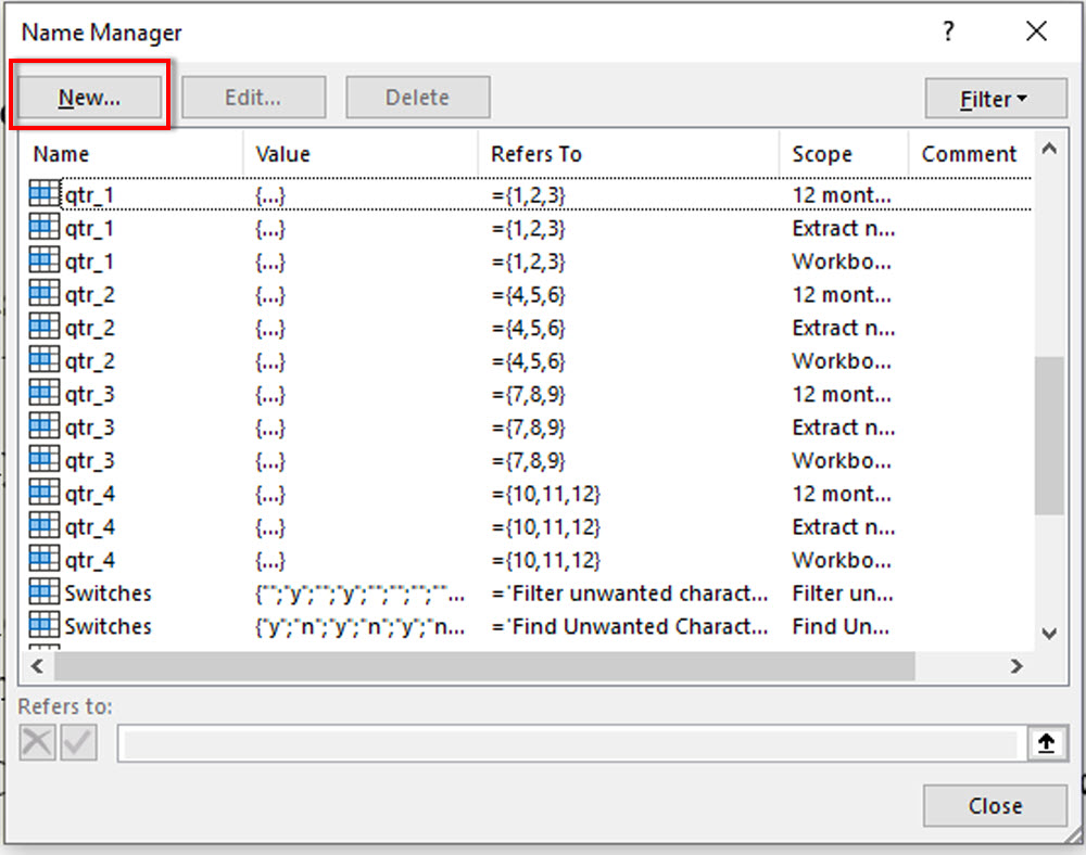
1.   Press CTRL+F3 to go to the Name Manager

          CTRL+F3: Opening the Name Manager

 

2.   Press Alt+N (or simply click the New… button) to define a new name

 

3.   In the New Name pane that opens, click: O (for One) in the name. Of course, you can choose any name. I chose the shortest 'cause I'm lazy 😊

 

4.     In the Refers to type: =INDEX!$A$1 (or: Sheet1!$A$1 or whatever the name of your master sheet is) and press: OK

Defining the shortcut to the INDEX worksheet

 

Now, from any worksheet, in order to navigate to the INDEX sheet, just:
1. CTRL+G (or F5) to open the go to pane

2. Type: O

3. Press: OK

                                 Fastest navigation to the target sheet

If you're nimble enough, you can do it in less than 200 milliseconds !!!!

Do you have a faster way?

 

 

 

תוכנה שפיתחתי ב"אקסל" – מתרגמת סכומים למילים בעברית

 

 

תוכנה שפיתחתי ב"אקסל" – מתרגמת סכומים למילים בעברית

רוצים לתרגם סכומים למילים בעברית?

תוכנה שפיתחתי ב"אקסל" מתרגמת סכומים לעברית:

משקל אחד ועד 999 מיליארד.

צפו בסרטון המצורף.

מעוניינים?

צרו אתי קשר בנייד המופיע בסרטון

אה, עיקר שכחתי:

חובה להדליק רמקולים 

https://www.youtube.com/watch?v=iUU712jJa2M

 

 

How to split a multi-line cell into separate cells

How to split a multi-line cell into separate cells?

There are at least two known solutions to this problem: splitting multiple lines within a cell to separate cells, each containing one line of the original, multiple-line cell.

1.    Text-to-Columns
This method uses the delimiter CTRL+J.
Typing these two keys together, creates the linefeed (hidden) character.

 

2.    Power Query

In Power Query, you choose:
Split Column->By Delimiter->split using special characters->

Insert special character->linefeed

 

But what I want to show you today is a method I've invented, which is (I believe) both the fastest and the simplest.
The solution can "materialize" thanks to the new TEXTSPLIT function in Excel 365 (I'm an "Office Insider" user but I believe that this function is already available to all 365 users, and if not, it will soon be).

So, without further ado let's dive into my solution.

1.    Our  multi-line cell looks like this (Cell A1):

     PIC 1: Cell A1 is multi-line and we want to split each line into a separate cell

 

 

2.    We define the delimiter. In cell I1 we type: =CHAR(10)

CHAR(10) is the ASCII linefeed character.

 

                                       PIC 2: defining the delimiter

 

3.    In cell B4, we type the following formula:

=TEXTSPLIT(A1, I1)

And the contents of cell A1 (5 lines) are split into 5 cells: B4-F4.

 

                                       PIC 3: splitting horizontally

 

And of course, we can split vertically as well:

 

                   PIC 4: splitting vertically

 

That's all, folks.

Hope you liked it.