This is C-r-a-z-y: SQRT instead of MATCH

 

This is C-r-a-z-y: SQRT instead of MATCH

I reckon you're all familiar with INDEX-MATCH. There's a myriad of video clips on Youtube with good, detailed explanations.

 

What I'm going to talk about is the: INDEX-MATCH-MATCH combination, where your search is two-dimensional: row (vertical) and column (horizontal).

So, actually you're looking for a solution which fulfills 2 conditions (criteria),
as demonstrated in the following pictures.

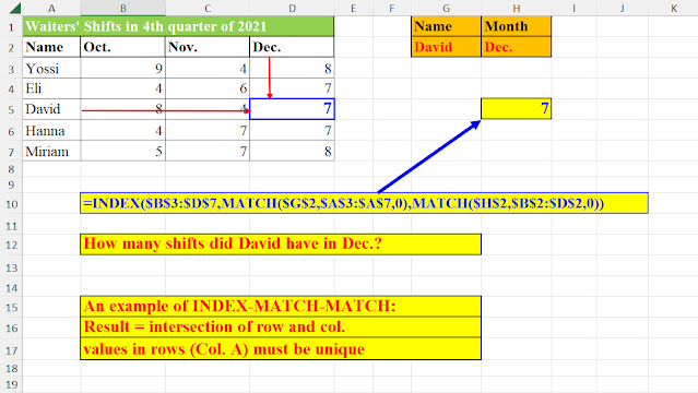
Example 1: How many shifts did David have in the month of December?

          Pic 1: INDEX-MATCH-MATCH - Example 1

  

 

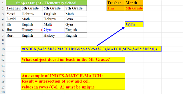
Example 2: What subject does Jim teach in the sixth Grade?

Pic 2: INDEX-MATCH-MATCH - Example 2

 

Example 3: What's Lara's score in Sports?

Pic 3: INDEX-MATCH-MATCH - Example 3

Now, let's move to a more complicated challenge. Here, instead of 2 conditions, one vertical (row) and one horizontal (column) we have 2 horizontal conditions.

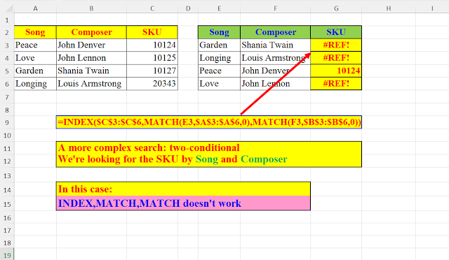
Consider the following dataset:
We are looking for the SKU by Song and composer. Actually, we are looking for the row in which these two meet.

But here the INDEX-MATCH-MATCH doesn't work.

Pic 4: INDEX-MATCH-MATCH - does not work

 

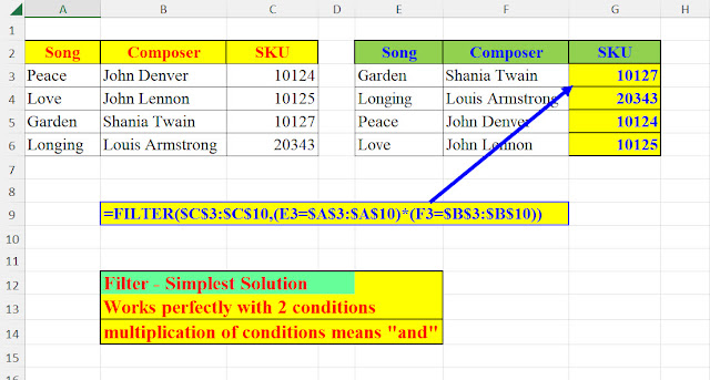
One possible solution is using the filter function, as can be seen in the picture below:

Pic 5: Using FILTER

 

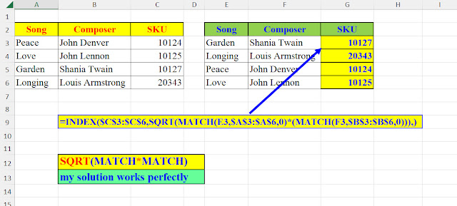
But, a small change to the original INDEX-MATCH-MATCH will make it operative and functioning: We add the SQRT function, and we also multiply both MATCH parts of the formula:

          Pic 6: Adding SQRT to INDEX-MATCH-MATCH – solves the problem

 

Amazing, but how does it work? Can you please explain?

How does it work?                                                                        

Since we're looking for an SKU where the Song and the Composer are on the same row,  then each of the two MATCH-es will yield the same number (i.e., row number).                                                                      

So, the multiplication of a number by itself gives us its square value.                          

What is left for us to do is to SQRT this number in order to find the row
So the solution is: INDEX(SQRT(MATCH(..)*MATCH(..)),)

Pic 7: Adding SQRT to INDEX-MATCH-MATCH - Explanation

 

Now, let's take a more complex situation where a song appears more than once.

With FILTER, the solution is very simple.

                                   Pic 8: A more complex scenario - solved by FILTER

Can this scenario be also solved with the previous method of
SQRT(MATCH(…)*MATCH(…))?

Well, not exactly, but basically: yes.

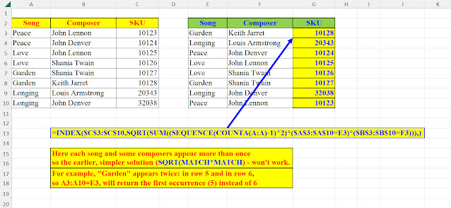
As I said, each composer and each song might appear more than once.

For example, "Garden" appears twice: in row 5 and in row 6,                             

so A3:A10=E3, will return the first occurrence (5) where we need the sixth occurrence (Garden with Keith Jarret, not: Garden with Shania Twain)                       
So we have to adapt our solution to the new situation.

 

And here's the solution to the more complex situation, still using
SQRT(MATCH(...)*MATCH(…))

Pic 9: A more complex scenario - solved by SQRT

 

Now we have to cater for cases of error (“not found”).

So, again, here are the three solutions.
2 “traditional” ones: FILTER & INDEX-MATCH
and the third one is the new SQRT….

 

Pic 10: FILTER - catering for “not found”

 

 

 

Pic 11: INDEX-MATCH - catering for “not found”

 

 

Pic 12: INDEX-SQRT - catering for “not found”

 

 

 

Creating a Dynamic Yearly Calendar

Creating a Dynamic Yearly Calendar

 

Using SEQUNCE, creating a dynamic yearly calendar is a piece of cake.

                              The Calendar

What it takes is only 5 easy steps:

1.     Add the year parameter (“yyyy”) in cell K1

 

2.     In cell A1, write the following formula:

=TEXT(WEEKDAY(SEQUENCE(,7)),"b1ddd")

 

3.     in cell A2, write the following formula:

 

=LET(d, DATE($K$1,1,1),SEQUENCE(54,7,1-WEEKDAY(d)+d))

 

4.     Select cells A2:G2, go to Conditional Formatting and add the following rule:

 

=A2<DATE($K$1,1,1)

 

Then, press the Format button, and in the Format cells pane, select Font and choose White background from the Color Dropdown

 

5.     Select cells A54:G55, go to Conditional Formatting and add the following rule:

 

=A54>DATE($K$1,12,31)

 

Then, press the Format button, and in the Format cells pane, select Font and choose White background from the Color Dropdown (same as in step 4.)

 

 

Conditional Formatting to hide unnecessary cells

 

That’s all.
Now you have a perfect calendar. If the year does not begin on Sunday, then the cells on row 2 preceding January 1^st will be empty.

The same applies to the end of the year: dates that occur after December 31^st will be empty.

 

 P.S.:

If you wonder why I used 54 weeks (instead of 53 weeks) in my solution, the reason is this:
A leap year has 366 days. So if it starts on Saturday and ends on Sunday, then we have 54 weeks. This happened, for example, in year 2000.

 

         

 

Three methods to find the n-largest/n-smallest number in one formula

 

3 methods to find the n-largest/n-smallest number in one formula

 

Suppose you want to find the n-th largest or n-smallest number in a list:

1^st largest, 2^nd largest or the 5^th smallest etc.

How can this be achieved with only one formula?
Answer: with parameters.
Parameter No.1: n (desired “location”) in cell D1

Parameter No.2: Largest (“T”) or Smallest (“B”) in cell F1

Here are three methods that apply this concept:

                             Method 1: LARGE & SMALL

                                      Method 2: LARGE only

 

                                 Method 3: AGGREGATE

 

 

Order of Adjectives in a Sentence

 

Order of Adjectives in a Sentence

- There are 10 categories of adjectives (see table below).

- If you want to modify a noun with more than one adjective, the order of these categories matters…

- Of course, having too many adjectives in one sentence is not recommended

  

 

Examples:

השימוש ב- would

 

השימוש ב- would

למילה would  ישנם הרבה שימושים באנגלית.

מספר דוגמאות:

1)     צורת העתיד-עבר (Future-Past) – אפשרות בעתיד שהחלה בעבר

 

·        He said he would finish his work by Monday

(yesterday he said: “I’ll finish my work by Monday”)

·        I thought he would be here by now

(An hour ago I thought: “I believe he will be here in an hour”)

 

2)     פעולות בשלילה בעבר (רצון או יכולת )

·        The car wouldn’t start this morning

(We tried to start the car, but we failed)

·        She wouldn’t get out of bed all day long
(She refused to get out of bed)

 

3)     סבירות גבוהה של משהו שקרה לפני זמן קצר

·        A: There was a knock at the door. Did you hear it?

B: Yes, that would be Bran Clark. He wants to join the club.

 

4)     בקשה נימוסית

·        Would you please stop that noise?

 

5)     בטוי רצון חזק

·        I would like to go to a restaurant tonight

 

6)     Would that (הלואי ש...)

·        A: If I won the lottery, I would travel to China

B: Would that it were so

 

 

7)     העדפת אפשרות אחת על אחרת (עם: sooner…. than/rather…than)

·        He’d (=He would) rather/sooner die than tell his wife the truth

 

8)     Conditional II (משפט תנאי – סבירות נמוכה)

·        If I won the money, I would invest it cleverly

 

9)     Conditional III (משפט תנאי – לא אפשרי/מצב בלתי-הפיך)

·        I would have passed the exam, if I had studied all day long

 

10) מצב היפותטי (לא מותנה)

·        She would be an amazing partner

 

11) דעה מנומסת

·        I would expect them to leave since they aren’t helping us

 

12) שאלה רטורית

·        Why would I lie to you?

 

13) עצה מנומסת

·        I wouldn’t go out with her, if I were you 

 

14) הצעה מנומסת

·        Would you like some more coffee?

Excel - Adding Superscript to Ordinal Numbers

 

Excel - Adding Superscript to Ordinal Numbers

If you use Word regularly, you probably know that whenever you want to specify an ordinal number (i.e., first, second, third…) all you have to do is add 2 letters to the cardinal number and Word automatically converts it into an ordinal number: you type 1st  and word changes it 1^st , 2nd  is transformed into 2^nd  etc.

But what about Excel?
Well, here the situation is much more complicated. In order to add these 2 superscript letters next to the number 1 (for example) you need 5 steps:

1.     Type “1st”

2.     Select “st”

3.     Press CTRL+1 (Format Cells)

4.     Check the Superscript checkbox

5.     Press the OK button

 

                   Pic 1: Adding superscript letters – the old way

 

Now, if you have many such ordinal numbers, this process might take a few minutes.
I’ve developed an alternative method which might save you some time.

It involves 3 steps which can automate the process of adding the superscript to the first 20 natural numbers with only one formula.

Step1:
Write the 6 formulae that appear in the picture. These are the 6 superscript letters that we use in all the ordinal numbers: st (for: 1^st ), nd (for 2^nd)

r (for 3^rd) and h (for 4^th,5^th…..20^th)

These formulae “convert” the Unicode of these letters to superscript letters.
The formulae create 6 superscript letters: “s” (in H2), “t” (in H3), “n” (in H4), “d” in (in H5), “r” (in H6) and “h” (in H7).

          Pic 2: Creating the 6 necessary Superscript Letters (H2:H7)

Step 2:

Combine the 4 pairs of letters that we use in all the ordinal number:
(st (for: 1^st ), nd (for 2^nd), rd (for 3^rd) and th (for 4^th,5^th…..20^th)

The result is shown in cells D1:D4

 

Pic 3: Creating 4 Pairs of Superscript Letters (D1:D4)

 

Step3:

Write the following Formula in cell A1 and drag it all the way down to cell A20:

=LET(x,ROW(),
SWITCH(x,1,x&$D$1,2,x&$D$2,3,x&$D$3,x&$D$4))

Pic 4: One Formula for the first 20 Ordinal Numbers