The ultimate Solution to cleaning Data
Amazing!
The Ultimate Solution!
No need for Power Query!!!
This
problem “pops up” in myriad Excel forums & groups:
How do I
“clean” my data?
How do I remove all non-printable characters from a cell?
Excel’s help (the TRIM & CLEAN functions) is very limited.
It cannot eliminate all those "hidden" characters.
The
perfect (and dynamic) solution is offered here, in a formula that I’ve
developed, as can be seen in the attached pictures.
The
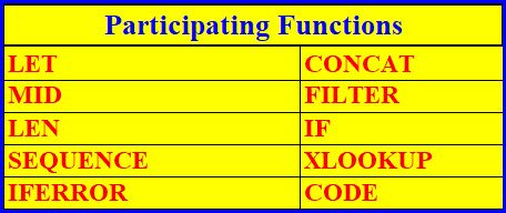
formula is quite complex and involves 10(!) Excel functions.

Participating Functions
The
solution enables us to choose (by parameters)
which characters we want to see in the “clean” result:
For example: digits (ASCII 48-57),
lower case English (ASCII 65-90),
upper case English (ASCII
97-122) etc..
Other subsets of the ASCII character set might change according
to locale. For example, in a Hebrew UI the Hebrew alphabet resides in
ASCII 224-250.
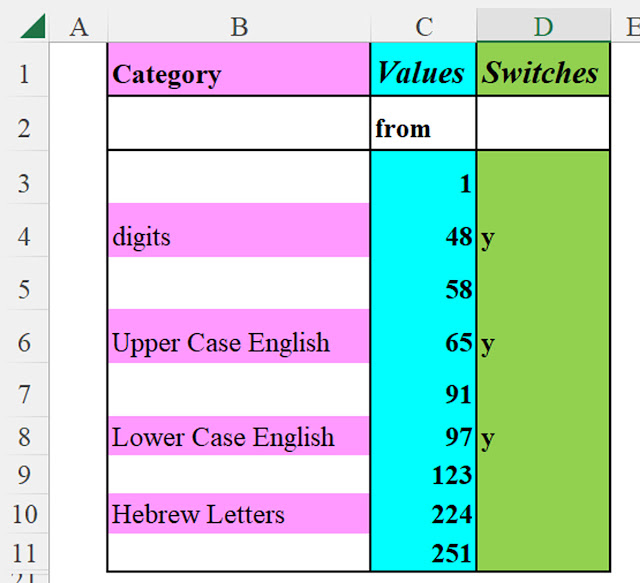
The Parameters Table
The parameters table enables you to define the groups of
characters (subsets of the whole ASCII character set) that you want in the "clean"
cells.
1. Each category's
value starts at the first value of that category. For example, the digits category's
is 48, since the digits are ASCII codes: 48-57.
2. By typing “y”
next to the desired subset, in column D, any group of characters: digits,
English (lower), English (upper) etc. or any combination of these
groups/subsets – is selected for the output result. Thus, you can dynamically control
which subset/s will appear in the "clean" cells, without
"tampering with" the formula. A category whose switch is "turned
off" (i.e., its value is not "y") – will be left outside of the
"clean" cells.
Two
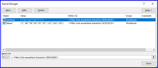
defined names (in the name manager) refer to the groups and the parameters.
Values
(i.e. groups/subsets) refer to cells C3:D11
Switches
(i.e. parameters) refer to cells D3:D11
as can be seen in the picture:
You are
free, of course, to add any subset you desire. For example: Special characters
(ASCII 33-47): ! " # $ % & ' ( ) *
+ , - . /
In my example, cells A27:A33
are the cells to be cleaned.
I chose to display only digits and English letters (both uppercase and
lowercase) in the "clean" cells.
Cells B27:B33
hold the “clean” data, which (according to the parameters) have only digits and
English letters (both uppercase and lowercase), as explained above.
The somewhat long formula 😊 is displayed here and refers to cell B27 (the "clean" result of cell A27).
=LET(s,MID(A27,SEQUENCE(LEN(A27)),1),IFERROR(CONCAT(FILTER(s,IF(XLOOKUP(CODE(s),Values, Switches,,
-1)="y",1,0))),""))
Double-click
the right lower corner of cell B27, to "spi the formula to the rest of the
range (B28:B33)
And here's
the final result:
The cells before (A27:A33) and after (B27:B33) cleaning
That’s all.
It is
desirable and even recommended to try at home.
Enjoy.


