Don’t use FIND/SEARCH, use this approach instead

 

Don’t use FIND/SEARCH, use this approach instead

Surprised by the article’s title?

Here’s the scenario:

You own a restaurant and you have some waiters working on 3 different shifts: morning, noon, evening.
You want to know, for a certain period of time (say: Sunday, Monday and Tuesday), how many assigned shifts did each waiter have during that period.

You might be tempted to do this:

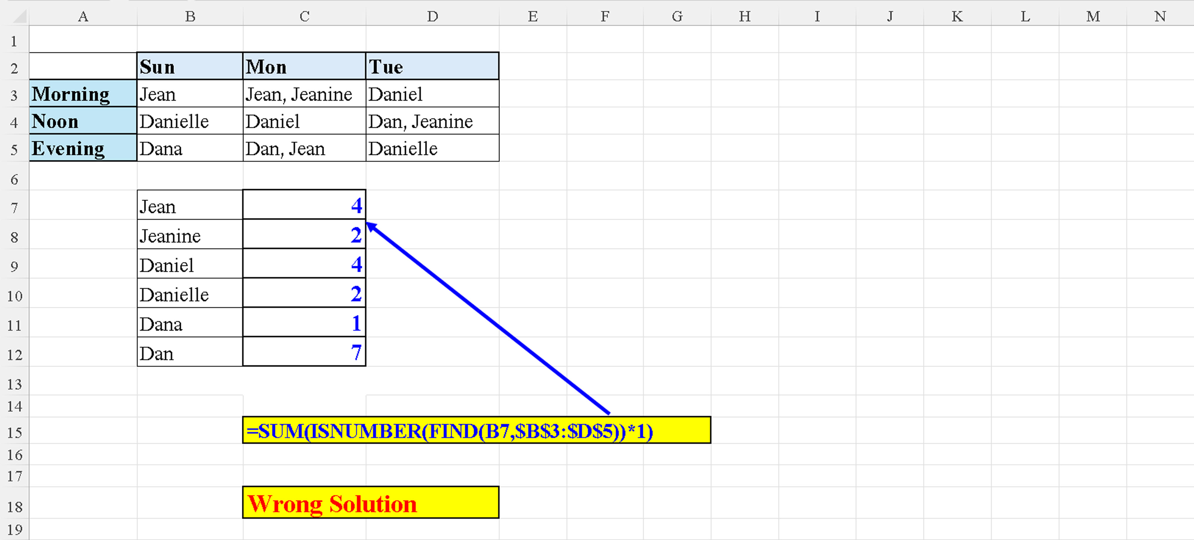
                   Pic 1: Wrong Solution

As can be seen clearly, this is a wrong solution:
Jean does not appear 4 times in the list, but only 3.
Dan does not appear 7 times in the list, but only twice.
So, what is the root of the problem?
The name “Jean”, for example, is contained within “Jeanine”. So the FIND function finds the substring “Jean” 4 times in the list.

The name “Dan” is contained in “Dana”, “Daniel” and “Danielle”, so the FIND function fetches all the instances of the substring “Dan” within the list.

Here we can see another shortcoming of the FIND function.
If, for example, we have “Jean” twice in cell C3, the formula:

=SUM(ISNUMBER(FIND(B7,C3)*1)

Will return a wrong result: 1 instead of 2.

FIND stops short of finding all the instances of the searched string within the cell.

                   Pic 2: Wrong Solution (a single cell)

 

So, you’d  probably ask, what is the solution to this problem?
The answer is: use EXACT instead of FIND.

The formula is a bit longer but by using the EXACT function we get the exact solution.

                   Pic 3: Correct Solution

 

 

And as a “bonus”, if the name “Jean” appears twice in cell C3, the EXACT function returns the correct result, unlike the FIND function (as demonstrated above):

                   Pic 4: Correct Solution (a single cell)

 

 

 

 

Combine data from multiple sheets without PQ

 

Combine data from multiple sheets without PQ

We all know that Power Query is the ideal tool to combine data from multiple tables/sheets/files etc.
But sometimes one can use a simpler, faster solution. This solution will still work even if the data changes.

Consider the following scenario:
I and some friends are planning on a four-day camp in the desert. We have prepared the list of products and quantities per product for each day. In order to buy these products, we need to find out the total quantity for each product that we are going to consume in our trip. Of course, some items might repeat themselves in several days. And of course, as stated above, we want the solution to be dynamic: if you add/delete a product, or if you modify a product’s quantity, we want this to be reflected in the purchase list.

So here’s the data, in 4 sheets: Day1 to Day4

                        Day 1: Products and Quantity

                        Day 2: Products and Quantity

 

 

                        Day 3: Products and Quantity

 

                        Day 4: Products and Quantity

 

We have two solutions, using VSTACK

Solution 1:
1) Create a dynamic array of all the data in all four sheets.
2) Use this array in a pivot table. All the “empty” rows of array are grouped into one row in the pivot table.

    The Pivot Table uses the array created by VSTACK

 

3) This “0” row of the Pivot Table can easily be eliminated by filtering it out.

        The Pivot Table after filtering out the “0” row

 

 

Solution 2:

Using both VSTACK and the new GROUPBY functions, we can achieve the same in one formula.
The same method may be employed to get rid of the “0” row (or even the “total” row if you omitted the 4^th argument to the GROUPBY function).

        VSTACK & GROUPBY instead of Power Query